在计算机辅助几何设计和计算机图形学中，采用光滑曲线拟合点云是一个广泛研究的问题(Várady等，1997)。通过激光扫描、X射线断层成像等先进采样设备获取测量数据，并对其进行数据拟合，可以实现对原模型进行大致的重建及功能恢复。但有些情况下，获取的数据点不仅是散乱的坐标信息，还包含一些约束形状的条件，如光学工程领域对带有法向约束的数据点的处理(胡巧莉和寿华好，2014; 胡良臣和寿华好，2016)。

与参数曲线相比，隐式曲线不需要对散乱数据点进行参数化就可以描述具有复杂集合形状的对象。传统的基于B样条的隐式曲线重构已有了一系列高效、快速和稳定的算法(Yang等，2005; Liu等，2017; Hamza等，2020)。Yang等人(2005)提出了一种基于B样条的隐式曲线重构模型，能够处理具有复杂拓扑结构的点云。Hamza等人(2020)将渐进迭代逼近法应用于隐式B样条曲线和曲面重建，提高了重建结果的质量，但是由于隐式B样条曲线的控制网格的控制顶点需要整行整列地规则排列，使得在局部细分方面存在一定的局限性，会造成控制点冗余现象。Sederberg等人(2003, 2004)提出了T样条方法，允许出现T节点，在继承B样条曲面优点的基础上，又增加了控制点较少、局部细分等优势，是一项很有前途的技术，在逆向工程等领域得到了广泛研究。在T样条拟合方面，Zheng等人(2005)首先提出了在z-map条件下的T样条曲面重构。Wang和Zheng(2007, 2013)将三角网格转化为T样条曲面，并提出了曲率引导下的T样条拟合方法。童伟华等人(2006)提出了隐式T样条曲面，将T网格从2维推广至3维，实现了曲面重构。唐月红等人(2011)提出一种新的隐式T样条曲面重建算法。近年来，一些快速拟合T样条的方法相继提出。Lin(2012)、Lin和Zhang(2013)将渐进T样条数据拟合算法用于拟合大数据集，迭代速度稳定，且不受未知T网格顶点数量增加的影响。Lu等人(2020)提出了基于区域分割的T样条拟合方法。

基于上述有关T样条的研究，本文将T样条函数应用于曲线重构问题，提出了一种带法向约束的隐式T样条曲线重构算法。通过结合曲率自适应地调整了采样点的疏密程度，利用加入曲线偏移点和光滑项消除额外零水平集，同时加入法向项约束曲线的法向方向，初步得到一条隐式T样条曲线。同时，优化了局部细分的算法，对曲线进行局部修正，在降低曲线误差的前提下，减少了插入控制系数的数量，最终得到一条满足数据点和法向约束的隐式T样条曲线。

若隐式曲线通过隐函数$f: \boldsymbol{\varOmega} \subset \mathbf{R}^{2} \rightarrow \mathbf{R}$，则称$\boldsymbol{S}=f^{-1}(0)=\{p \in \boldsymbol{\varOmega}; f(p)=0\}$ 为隐式曲线。若函数$ f$为T样条函数，则隐式曲线$\boldsymbol{S} $称为隐式T样条曲线。

定义在2维T网格上的隐式T样条曲线方程为

$ f(x, y)=\frac{\sum\limits_{i=1}^{m} c_{i} B_{i}(x, y)}{\sum\limits_{i=1}^{m} B_{i}(x, y)}=0,(x, y) \in \boldsymbol{\varOmega} $

(1)

式中，$c_{i}$是控制系数。控制系数$c_{i}$对应的T样条基函数$B_{i}(x, y)$为

$ B_{i}(x, y)=N\left[\boldsymbol{s}_{i}\right](x) N\left[\boldsymbol{t}_{i}\right](y) $

(2)

式中，$N\left[\boldsymbol{s}_{i}\right](x)$和$N\left[\boldsymbol{t}_{i}\right](y)$是三次B样条基函数，相应的节点向量为$\boldsymbol{s}_{i}=\left[s_{i 0}, s_{i 1}, \cdots, s_{i 4}\right]$和$\boldsymbol{t}_{i}=\left[t_{i 0}, t_{i 1}, \cdots, t_{i 4}\right]$。此时，$N\left[\boldsymbol{s}_{i}\right](x)$可表示为

$ \begin{array}{c} N\left[\boldsymbol{s}_{i}\right](x)= \\ \begin{cases}\frac{1}{a_{0}} A_{0}(x) & x \in\left[s_{i 0}, s_{i 1}\right) \\ \frac{1}{b_{0}} B_{0}(x)+\frac{1}{b_{1}} B_{1}(x)+\frac{1}{b_{2}} B_{2}(x) & x \in\left[s_{i 1}, s_{i 2}\right) \\ \frac{1}{c_{0}} C_{0}(x)+\frac{1}{c_{1}} C_{1}(x)+\frac{1}{c_{2}} C_{2}(x) & x \in\left[s_{i 2}, s_{i 3}\right) \\ \frac{1}{d_{0}} D_{0}(x) & x \in\left[s_{i 3}, s_{i 4}\right) \\ 0 & \text { 其他 }\end{cases} \end{array} $

式中，

$ \left\{\begin{array}{l} a_{0}=\left(s_{i 1}-s_{i 0}\right)\left(s_{i 2}-s_{i 0}\right)\left(s_{i 3}-s_{i 0}\right) \\ b_{0}=-\left(s_{i 2}-s_{i 1}\right)\left(s_{i 3}-s_{i 0}\right)\left(s_{i 2}-s_{i 0}\right) \\ b_{1}=-\left(s_{i 2}-s_{i 1}\right)\left(s_{i 3}-s_{i 1}\right)\left(s_{i 3}-s_{i 0}\right) \\ b_{2}=-\left(s_{i 2}-s_{i 1}\right)\left(s_{i 4}-s_{i 1}\right)\left(s_{i 3}-s_{i 1}\right) \\ c_{0}=\left(s_{i 3}-s_{i 2}\right)\left(s_{i 3}-s_{i 1}\right)\left(s_{i 3}-s_{i 0}\right) \\ c_{1}=\left(s_{i 3}-s_{i 2}\right)\left(s_{i 4}-s_{i 1}\right)\left(s_{i 3}-s_{i 1}\right) \\ c_{2}=\left(s_{i 3}-s_{i 2}\right)\left(s_{i 4}-s_{i 2}\right)\left(s_{i 4}-s_{i 1}\right) \\ d_{0}=-\left(s_{i 4}-s_{i 3}\right)\left(s_{i 4}-s_{i 2}\right)\left(s_{i 4}-s_{i 1}\right) \end{array}\right. $

$ \left\{\begin{array}{l} A_{0}(x)=\left(x-s_{i 0}\right)^{3} \\ B_{0}(x)=\left(x-s_{i 0}\right)^{2}\left(x-s_{i 2}\right) \\ B_{1}(x)=\left(x-s_{i 0}\right)\left(x-s_{i 1}\right)\left(x-s_{i 3}\right) \\ B_{2}(x)=\left(x-s_{i 1}\right)^{2}\left(x-s_{i 4}\right) \\ C_{0}(x)=\left(x-s_{i 0}\right)\left(x-s_{i 3}\right)^{2} \\ C_{1}(x)=\left(x-s_{i 1}\right)\left(x-s_{i 3}\right)\left(x-s_{i 4}\right) \\ C_{2}(x)=\left(x-s_{i 2}\right)\left(x-s_{i 4}\right)^{2} \\ D_{0}(x)=\left(x-s_{i 4}\right)^{3} \end{array}\right. $

由式(1)确定的二元函数$f(x, y)$称为隐式T样条函数，由$f^{-1}(0)$定义的曲线称为隐式T样条曲线。

给定$n$ 个2维空间中的散乱数据点集$\boldsymbol{P}= \left\{\boldsymbol{p}_{i}=\left(x_{i}, y_{i}\right), i=1, 2, \cdots, n\right\}$, 且每个数据点带有一个有向的单位法向量$\boldsymbol{N}=\left\{\boldsymbol{n}_{i}, i=1, 2, \cdots, n\right\}$，现在需要找到一条隐式T样条曲线$f(x, y)$=0逼近给定的数据点且对于数据点在曲线上的对应位置满足法向约束条件，即$f\left(x_{i}, y_{i}\right)=0$且$\nabla f\left(x_{i}, y_{i}\right)= \boldsymbol{n}_{i}, i=1, 2, \cdots, n$。为了避免平凡解$ f$=0，在数据点集中加入一些额外的偏移点作为辅助点$\left\{\boldsymbol{p}_{l}=\right. \left.\left(x_{l}, y_{l}\right), l=n+1, n+2, \cdots, N\right\}$。假定$d_{l}$为偏移点$\boldsymbol{p}_{l}$到曲线上最近点$\boldsymbol{p}_{k}$的有向距离，即$\boldsymbol{p}_{l}=\boldsymbol{p}_{k}+d_{l} \boldsymbol{n}_{k}$，此时隐函数在偏移点处的方程为

$ f\left(x_{l}, y_{l}\right)=d_{l}, l=n+1, n+2, \cdots, N $

(3)

令$\boldsymbol{v}_{i}$表示曲线在$\boldsymbol{p}_{i}$处的单位切向量，显然

$ \boldsymbol{v}_{i} \cdot \boldsymbol{n}_{i}=0, i=1,2, \cdots, n $

由此可以得到$n$ 个单位切向量$\boldsymbol{v}_{i}$的值。于是问题转化为要求函数$ f$满足

$ \begin{cases}f\left(x_{i}, y_{i}\right)=0 & i=1,2, \cdots, n \\ f\left(x_{i}, y_{i}\right)=d_{i} \neq 0 & i=n+1, n+2, \cdots, N \\ \nabla f\left(x_{i}, y_{i}\right) v_{i}=0 & i=1,2, \cdots, n\end{cases} $

(4)

隐式T样条曲线重构算法步骤如下：

输入：散乱数据点集$\boldsymbol{p}_{i}$和对应的单位法向量$\boldsymbol{n}_{i}, i=1, 2, \cdots, n$。

输出：T网格和网格点对应的控制系数。

1) 对输入的数据进行预处理，通过曲率自适应调整采样点的疏密程度，利用单位法向量加入偏移点作为辅助点，同时求出每个数据点的单位切向量。

2) 利用二叉树对数据点进行细分，自动生成合理的2维T网格。给T网格的每条边赋予一个节点区间值，同时给T网格的边界加入相应的虚边, 并给虚边赋予一个非负值。

3) 利用T网格获取网格上每个点的局部坐标系，从而得到每个控制系数对应的节点向量，进而得到T样条基函数。

4) 建立合适的优化模型，并用最小二乘法求得T样条的控制系数，获得隐式T样条曲线。

5) 对得到的隐式T样条曲线与给定的数据点集和单位法向量进行分析，判断是否达到精度要求。在误差较大的区域插入新的控制系数进行修正，然后更新节点向量，转步骤4)，直到满足精度要求。

将隐式T样条应用到曲线重建的关键问题是构造合理的2维T网格，使其控制系数满足一定的拓扑关系。

T样条是允许出现T节点的矩形网格，控制网格的顶点不要求整行整列的排列，因此构造T网格可以在数据点密集的地方多插入控制系数，在数据点稀疏的地方少插入控制系数，使T网格的网格点的数量相比B样条的控制网格大幅减少，在保证类似精度的前提下提高了重建曲线的效率。在2维平面上利用二叉树方法进行细分的步骤如下：

1) 定义一个细分的最大次数和一个阈值，其中，阈值表示每个矩形块中允许包含的最大点数。

2) 计算每个矩形块中包含的数据点数量，若某个矩形块包含的数据点个数大于给定的阈值，则对其进行细分。具体来说，假定该矩形块的左下角坐标为$\left(s_{\text {min }}, t_{\min }\right)$，右上角坐标为$\left(s_{\max }, t_{\max }\right)$，T网格$ s$方向的长度为$s_{m}, t$方向的长度为$t_{m} $。如果$\left(s_{\max }-\right.$ $\left.s_{\text {min }}\right) / s_{m} \geqslant\left(t_{\text {max }}-t_{\text {min }}\right) / t_{m}$，那么在矩形块$s= \left[\left(s_{\text {max }}+s_{\text {min }}\right) / 2\right]$ 处将矩形块分成两块; 否则，在$t= [\left.\left(t_{\max }+t_{\min }\right) / 2\right]$ 处细分矩形块。

3) 重复步骤2)，直到每个矩形块包含的点数小于阈值或者达到最大的细分次数。

4) 输出细分后得到的T网格。

通过细分得到的T网格，不仅要保存T网格每个顶点的坐标，还需要通过节点区间值得到每个顶点对应的局部坐标系。

图 1是由一条封闭曲线构造的T网格。其中图 1(a)是曲线的初始采样点，包含466个数据点，图 1(b)是通过平面二叉树细分生成的2维T网格，包含131个网格点。

构造2维T网格后，因为每个控制系数$c_{i}$都对应T网格上的各个网格顶点，因此可以得到控制系数$c_{i}$的数量。然后通过T网格获得每个控制系数对应的节点向量$\boldsymbol{s}_{i}$和$\boldsymbol{t}_{i}$，从而确定控制系数的基函数。本文在构造T网格后，保存了网格顶点、边、节点区间值以及每个小矩形块的信息，以便对T网格进行局部修正。

通过T网格构造，得到每个控制系数对应的基函数后，尚需找到合适的隐式T样条函数$ f$满足式(4)中的条件。显然，待求的未知数即控制系数的数量远少于条件中给出的方程的个数，因此需要建立合适的优化模型，从而找到在某种意义下的最优解。此时，隐式曲线重构问题转化为最小值优化问题，得到的目标方程为

$ E_{\mathrm{fit}}(\boldsymbol{c})=E_{p}(\boldsymbol{c})+\omega_{1} E_{N}(\boldsymbol{c})+\omega_{2} E_{G}(\boldsymbol{c}) $

(5)

式中，$\boldsymbol{c}=\left[c_{1}, c_{2}, \cdots, c_{m}\right]^{\mathrm{T}}$为T网格中待求的控制系数，$E_{p}(\boldsymbol{c})$表示拟合误差平方和; $E_{N}(\boldsymbol{c})$表示法向项，$\omega_{1}$为法向项权值; $E_{G}(\boldsymbol{c})$表示光滑项，$\omega_{2}$为光滑项系数。这里，$E_{p}(\boldsymbol{c})$可以表示为

$ \begin{aligned} E_{p}(\boldsymbol{c})=& \sum\limits_{j=1}^{n}\left[f\left(\boldsymbol{p}_{j}\right)\right]^{2}+\sum\limits_{j=n+1}^{N}\left[f\left(\boldsymbol{p}_{j}\right)-d_{j}\right]^{2}=\\ & \boldsymbol{c}^{\mathrm{T}} \boldsymbol{L}^{\mathrm{T}} \boldsymbol{L} \boldsymbol{c}-2 \boldsymbol{c}^{\mathrm{T}} \boldsymbol{H}+\sum\limits_{j=n+1}^{N} d_{i}^{2} \end{aligned} $

式中，矩阵$\boldsymbol{L}=\left(l_{s t}\right)_{N \times m}, l_{s t}$表示为$B_{t}\left(x_{s}, y_{s}\right)$。$\boldsymbol{H}$是一个$m \times 1$的向量，它的每一项$h_{i}=\sum\limits_{j=n+1}^{N} d_{j} B_{i}\left(x_{j}\right., \left.y_{j}\right), i=1, 2, \cdots, m$。

$E_{N}(\boldsymbol{c})$可以表示为

$ \begin{gathered} E_{N}(\boldsymbol{c})=\sum\limits_{j=1}^{n}\left[\nabla f\left(\boldsymbol{p}_{j}\right) \cdot \boldsymbol{v}_{j}\right]^{2}= \\ \sum\limits_{j=1}^{n}\left[f_{x}\left(\boldsymbol{p}_{j}\right) \cdot v_{j x}+f_{y}\left(\boldsymbol{p}_{j}\right) \cdot v_{j y}\right]^{2}= \\ \boldsymbol{c}^{\mathrm{T}} \boldsymbol{A}_{x}^{\mathrm{T}} \boldsymbol{A}_{x} \boldsymbol{c}+2 \boldsymbol{c}^{\mathrm{T}} \boldsymbol{A}_{x}^{\mathrm{T}} \boldsymbol{A}_{y} \boldsymbol{c}+\boldsymbol{c}^{\mathrm{T}} \boldsymbol{A}_{y}^{\mathrm{T}} \boldsymbol{A}_{y} \boldsymbol{c} \end{gathered} $

式中，$\nabla f$表示函数$ f$的梯度，$ f_x$和$ f_y$分别表示函数$ f$对$x$和$y$求偏导数，$\boldsymbol{v}_{j}=\left(v_{j x}, v_{j y}\right)^{\mathrm{T}}$为数据点$\boldsymbol{p}_{j}$对应的单位切向量。而矩阵$\boldsymbol{A}_{x}=\left(a_{x}\right)_{n \times m}, \boldsymbol{A}_{y}= \left(a_{y}\right)_{n \times m}$，其中，矩阵$\boldsymbol{A}_x$的元素为$\left(a_{x}\right)_{s t}= \frac{\partial B_{t}\left(x_{s}, y_{s}\right)}{\partial x} v_{t x}, \boldsymbol{A}_{y}$的元素为$\left(a_{y}\right)_{s t}=\frac{\partial B_{t}\left(x_{s}, y_{s}\right)}{\partial y} v_{t y}$, $s=1, 2, \cdots, n, t=1, 2, \cdots, m$。

$E_{G}(\boldsymbol{c})$可以表示为

$ \begin{gathered} E_{G}(\boldsymbol{c})=\sum\limits_{j=1}^{n}\left[f_{x x}^{2}\left(x_{j}, y_{j}\right)+2 f_{x y}^{2}\left(x_{j}, y_{j}\right)+\right. \\ \left.f_{y y}^{2}\left(x_{j}, y_{j}\right)\right]= \\ \boldsymbol{c}^{\mathrm{T}} \boldsymbol{O}^{\mathrm{T}} \boldsymbol{O} \boldsymbol{c}+2 \boldsymbol{c}^{\mathrm{T}} \boldsymbol{P}^{\mathrm{T}} \boldsymbol{P} \boldsymbol{c}+\boldsymbol{c}^{\mathrm{T}} \boldsymbol{Q}^{\mathrm{T}} \boldsymbol{Q} \boldsymbol{c} \end{gathered} $

式中，$ f_{xx}$和$ f_{yy}$分别表示函数$ f$对$x$和$y$求二次偏导数，$ f_{xy}$表示函数$ f$的二阶混合偏导数。矩阵$\boldsymbol{O}= \left(o_{s t}\right)_{n \times m}, \boldsymbol{P}=\left(p_{s t}\right)_{n \times m}, \boldsymbol{Q}=\left(q_{s t}\right)_{n \times m}$，3个矩阵中的元素分别为$o_{s t}=\frac{\partial^{2} B_{t}\left(x_{s}, y_{s}\right)}{\partial x^{2}}, p_{s t}=\frac{\partial^{2} B_{t}\left(x_{s}, y_{s}\right)}{\partial x \partial y}$, $ q_{s t}=\frac{\partial^{2} B_{t}\left(x_{s}, y_{s}\right)}{\partial y^{2}}, s=1, 2, \cdots, n, t=1, 2, \cdots, m $。

为了求解优化问题，将式(5)的目标函数对控制系数c的每个分量求偏导，并使其等于零，即

$ \frac{\partial E_{\mathrm{fit}}(\boldsymbol{c})}{\partial c_{k}}=0, k=1,2, \cdots, m $

(6)

此时，问题转化为求解

$ \begin{gathered} {\left[\boldsymbol{L}^{\mathrm{T}} \boldsymbol{L}+\omega_{1}\left(\boldsymbol{A}_{x}^{\mathrm{T}} \boldsymbol{A}_{x}+\boldsymbol{A}_{x}^{\mathrm{T}} \boldsymbol{A}_{y}+\boldsymbol{A}_{y}^{\mathrm{T}} \boldsymbol{A}_{x}+\boldsymbol{A}_{y}^{\mathrm{T}} \boldsymbol{A}_{y}\right)+\right.} \\ \left.\omega_{2}\left(\boldsymbol{O}^{\mathrm{T}} \boldsymbol{O}+\boldsymbol{P}^{\mathrm{T}} \boldsymbol{P}+\boldsymbol{Q}^{\mathrm{T}} \boldsymbol{Q}\right)\right] \boldsymbol{c}=\boldsymbol{H} \end{gathered} $

(7)

解该线性方程组即可得到T网格中控制系数的值，从而得到隐式T样条曲线。

通过拟合模型得到一条隐式T样条曲线后，对拟合结果进行检测。采用$\Delta_{p_{i}}=\frac{\left|f\left(\boldsymbol{p}_{i}\right)\right|}{\left\|\nabla f\left(\boldsymbol{p}_{i}\right)\right\|}$ 计算每个采样点$\boldsymbol{p}_{i}$的拟合误差，用$\Delta_{n i}= \arccos \left(\frac{\nabla f\left(\boldsymbol{p}_{i}\right) \cdot \boldsymbol{n}_{i}}{\left\|\nabla f\left(\boldsymbol{p}_{i}\right)\right\|}\right)$ 计算隐式T样条曲线在采样点$\boldsymbol{p}_{i}$处的法向与给定的法向约束的误差，此时$\Delta_{i}= \Delta_{p_{i}}+\lambda \cdot \Delta_{n i}$表示曲线在$\boldsymbol{p}_{i}$处的总误差，其中$ \lambda $表示数据点误差和法向误差之间的权重关系。局部细分算法的具体步骤如下：

1) 给定一个容许误差$ \sigma $>0，细分比率$\alpha $和一个阈值$z$，这里的阈值小于上面构造T网格时给定的阈值。

2) 计算每个采样点$\boldsymbol{p}_{i}$对应的误差$\Delta_{i}$，若所有采样点的误差均小于容许误差$ \sigma $，则此时的隐式T样条曲线即为最终的曲线，循环终止; 否则，找到误差不满足的采样点处于哪些矩阵块后，执行步骤3)。

3) 计算需要细分的矩形块中包含的数据点的数量，若某矩形块的数据点数量小于给定阈值$z$，则将该矩形块排除需要细分的序列。

4) 统计需要细分的矩形块的总数量，与细分比率$\alpha $相乘，得到的值μ即为实际细分的数量。根据矩形块包含数据点的最大误差对矩形块从大到小进行排序，此时，对前μ个矩形块细分。

5) 更新T样条基函数，重新反求控制系数，得到新的隐式T样条曲线。

6) 重复步骤2)—5)，直到循环结束，输出T网格和相应的控制系数。

选取3个封闭曲线实例对隐式T样条曲线重建算法的性能进行验证。首先结合曲率自适应地调整采样点的疏密程度，然后进行曲线重构。现有的T样条重构的方法大多集中在曲面上，实验时，选取童伟华等人(2006)和唐月红等人(2011)的隐式T样条曲面重构方法用于隐式T样条曲线重建，分别作为方案1和方案2，其中，方案1通过添加隐函数对$x$, $y$求偏导分别等于法向分量的方程避免奇异解，重构隐式T样条函数; 方案2通过添加偏移点构造隐式函数。然后将两种方案与本文算法进行比较，以验证本文方法的性能。图 2展示了方案1和本文方法对3条曲线的重建，其中，图 2(a)是初始采样点显示的曲线，图 2(b)是构造的2维T网格，图 2(c)和图 2(d)分别为方案1和本文方法重构的曲线。可以看出，虽然本文方法和方案1都重构出了隐式T样条曲线，但是方案1的方法会产生一些额外的零水平集，破坏了重构效果。

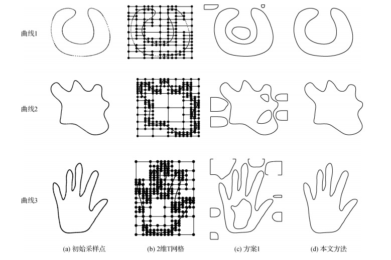
本文方法与方案1和方案2的定量比较结果如表 1所示。可以看出，3种方法在数据点处的误差相差不大，但是本文方法在法向误差处无论是平均误差还是最大误差都是最小的。方案1虽然也能约束法向，但是误差没有本文方法小，同时会产生零水平集。方案2重构曲率变化较小的曲线时，法向误差与方案1差不多，但在实现曲率变化较大的曲线，如曲线3的手型曲线时不能有效地约束法向，法向误差较大。本文对输入的数据点要求采样密集，当数据点比较稀疏时，对曲线1这种比较简单的曲线影响不大，但对比较复杂的曲线在曲率变化较大的位置无法较好地约束法向误差。

在网格顶点数量方面，隐式B样条需要大量多余的控制点来满足拓扑约束，而隐式T样条曲线可以大幅减少多余的网格点的数量。表 2给出了3条曲线关于B样条网格与T网格顶点数的比较，其中包括每个曲线采样的数据点数、网格在两个方向上的节点数以及控制顶点数。可以看出，3条曲线的T网格顶点数均小于B样条控制点数，从而大幅减少了运算量。

本文针对带有法向约束的离散数据点集提出了一种有效的隐式T样条曲线重建算法，较好地实现了3个封闭曲线实例的重建。实验结果表明，通过加入曲线偏移点作为辅助点和在拟合模型中加入光滑项，本文方法成功消除了额外零水平集，提高了重构曲线的质量。此外，通过在模型中加入法向项约束，重构的曲线会在逼近数据点的同时满足数据点处的法向约束。本文还优化了局部细分的算法，引入了细分比率这一概念，减少了插入控制系数的数量，提高了运算速度。本文将两种隐式T样条曲面重构的方法应用到曲线重构上，然后与本文的隐式T样条曲线重构方法进行比较。可以发现，在数据点误差精度相差不大的情况下，本文方法在法向误差精度上有了显著提高，而法向误差在光学反射曲线曲面设计等领域有着重要作用。本文将隐式T样条曲线的网格与隐式B样条的网格顶点数量进行比较，在两种控制网格的相同位置插入控制点时，由于隐式B样条曲线的网格需要大量多余的控制点来满足拓扑约束，实验结果显示，隐式T样条的网格顶点数只有B样条网格的一半左右。

总之，实验数据和重建的效果图显示，本文方法较好地解决了带法向约束的隐式T样条曲线重建问题。但本文方法仍有不足之处: 1)本文方法在重建不光滑的曲线如心形线时，在尖锐点的附近无法对法向进行有效约束，有较大的误差; 2)本文方法对数据点要求密集，若数据点比较稀疏，则在曲线曲率变化较大的位置将无法较好地约束法向误差。有待进一步研究。